In an era where digital presence is vital for business continuity, the concept of high availability (HA) has become a cornerstone in system design. High availability refers to systems that can operate continuously without failure for extended periods.
This article explores the evolution of high availability, how it is measured, how it is implemented in various systems, and the trade-offs involved in achieving it.
The concept of high availability originated in the 1960s and 1970s with early military and financial computing systems that needed to be reliable and fault tolerant.
In the Internet age, there has been an explosion of digital applications for e-commerce, payments, delivery, finance, and more. Positive user experiences are crucial for business success. This escalated the need for systems with nearly 100% uptime to avoid losing thousands of users for even brief periods. For example, during a promotional flash sale event, just one minute of downtime could lead to complete failure and reputation damage.
The goal of high availability is to ensure a system or service is available and functional for as close to 100% of the time as possible. While the terms high availability and uptime are sometimes used interchangeably, high availability encompasses more than just uptime measurements.
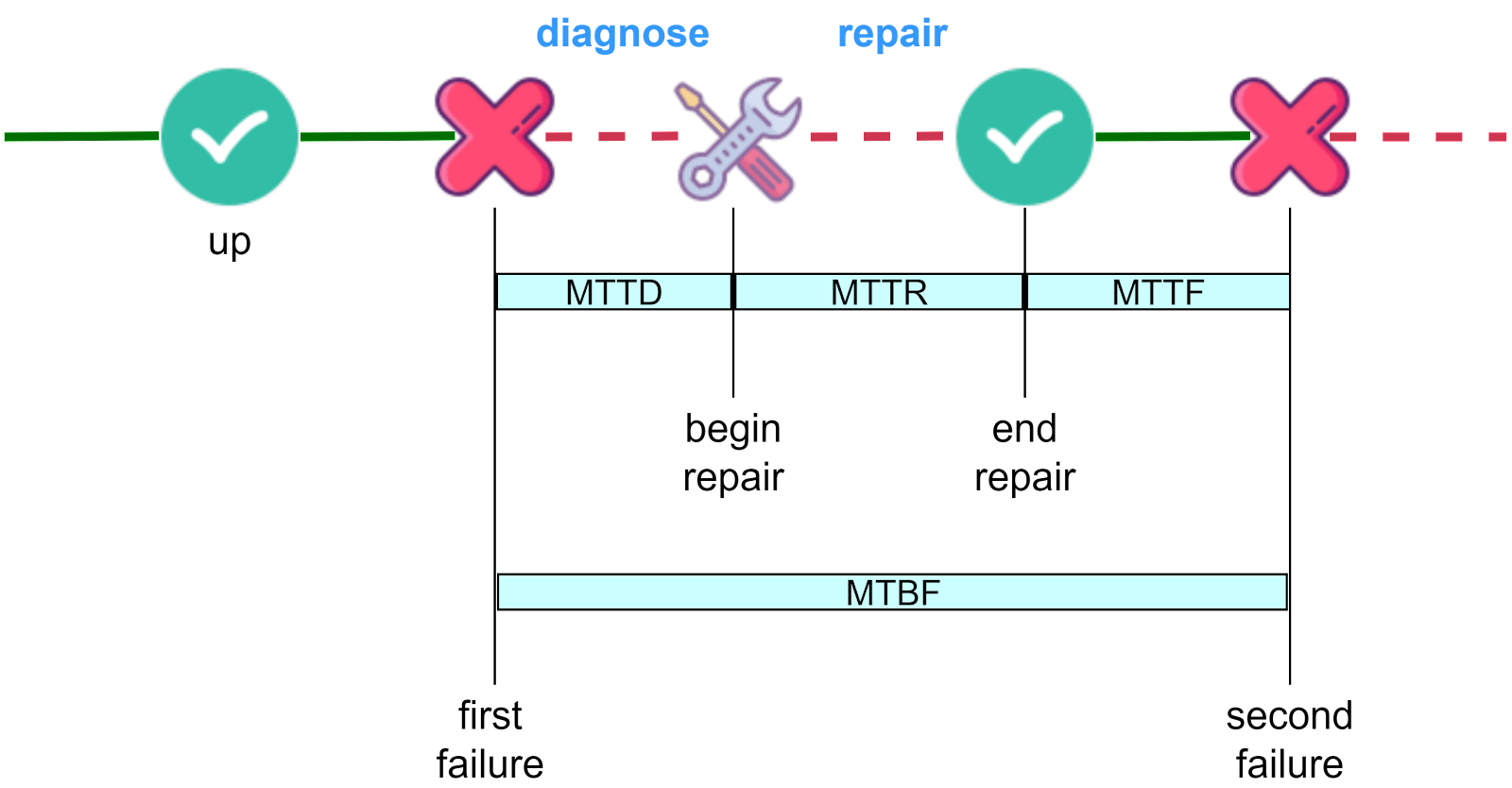
Two key concepts are relevant for calculating availability: Mean Time Between Failures (MTBF), and Mean Time To Repair (MTTR).
MTBF measures system reliability by totaling a system’s operational time and dividing it by the number of failures over that period. It is typically expressed in hours. A higher MTBF indicates better reliability.
MTTR is the average time required to repair a failed component or system and return it to an operational state. It includes diagnosis time, spare part retrieval, actual repair, testing, and confirmation of operation. MTTR is also typically measured in hours.
As shown in the diagram below, there are two additional related metrics - MTTD (Mean Time To Diagnose) and MTTF (Mean Time To Failure). MTTR can loosely include diagnosis time.
Together, MTBF and MTTR are critical for calculating system availability. Availability is the ratio of total operational time to the sum of operational time and repair time. Using formulas:
Availability=MTBFMTBF+MTTR
For high-availability systems, the goal is to maximize MTBF (less frequent failures) and minimize MTTR (fast recovery from failures). These metrics help teams make informed decisions to improve system reliability and availability.
As shown in the diagram below, calculated availability is often discussed in terms of “nines”. Achieving “3 nines” availability allows only 1.44 minutes of downtime per day - challenging for manual troubleshooting. “4 nines” allows only 8.6 seconds of downtime daily, requiring automatic monitoring, alerts, and troubleshooting. This adds requirements like automatic failure detection and rollback planning in system designs.

To achieve “4 nines” availability and beyond, we must consider:
System designs - designing for failure using:
Redundancy
Tradeoffs
System operations and maintenance - key principles are:
Change management
Capacity management
Automated detection and troubleshooting
Let’s explore system designs in more detail.
There is only so much we can do to optimize a single instance to be fault-tolerant. High availability is often achieved by adding redundancies. When one instance fails, others take over.
For stateful instances like storage, we also need data replication strategies.
Let's explore common architectures with different forms of redundancy and their tradeoffs.
In the hot-cold architecture, there is a primary instance that handles all reads and writes from clients, as well as a backup instance. Clients interact only with the primary instance and are unaware of the backup. The primary instance continuously synchronizes data to the backup instance. If the primary fails, manual intervention is required to switch clients over to the backup instance.
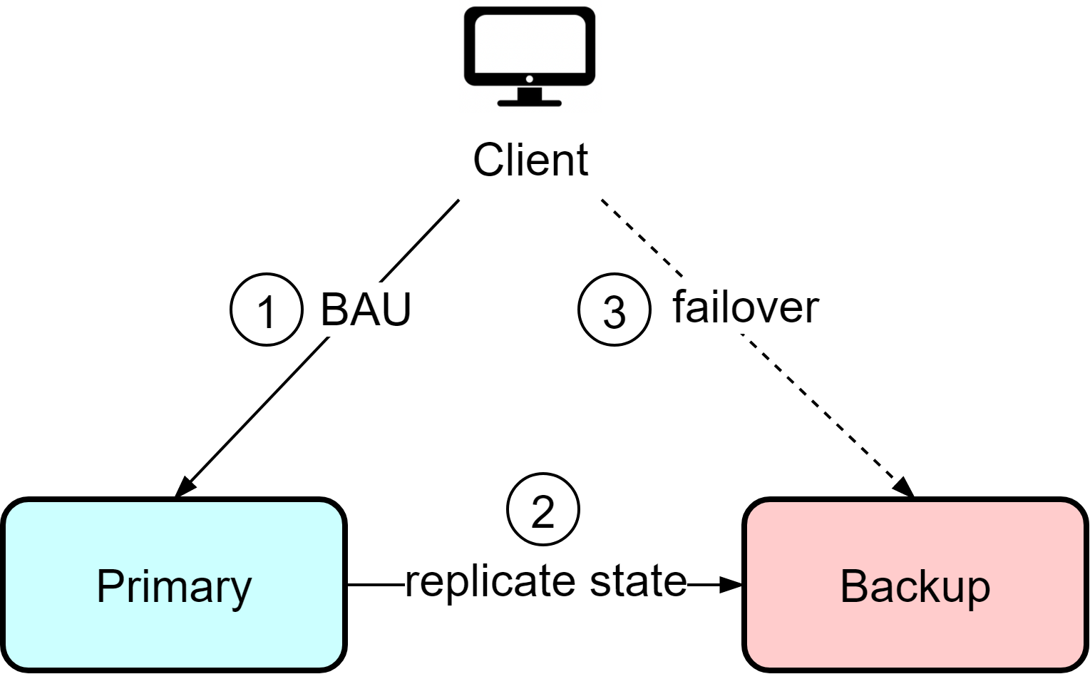
This architecture is straightforward but has some downsides. The backup instance represents waste resources since it is idle most of the time. Additionally, if the primary fails, there is potential for data loss depending on the last synchronization time. When recovering from the backup, manual reconciliation of the current state is required to determine what data may be missing. This means clients need to tolerate potential data loss and resend missing information.
The hot-cold architecture wastes resources since the backup instance is under-utilized. The hot-warm architecture optimizes this by allowing clients to read from the secondary/backup instance. If the primary fails, clients can still read from the secondary with reduced capacity.
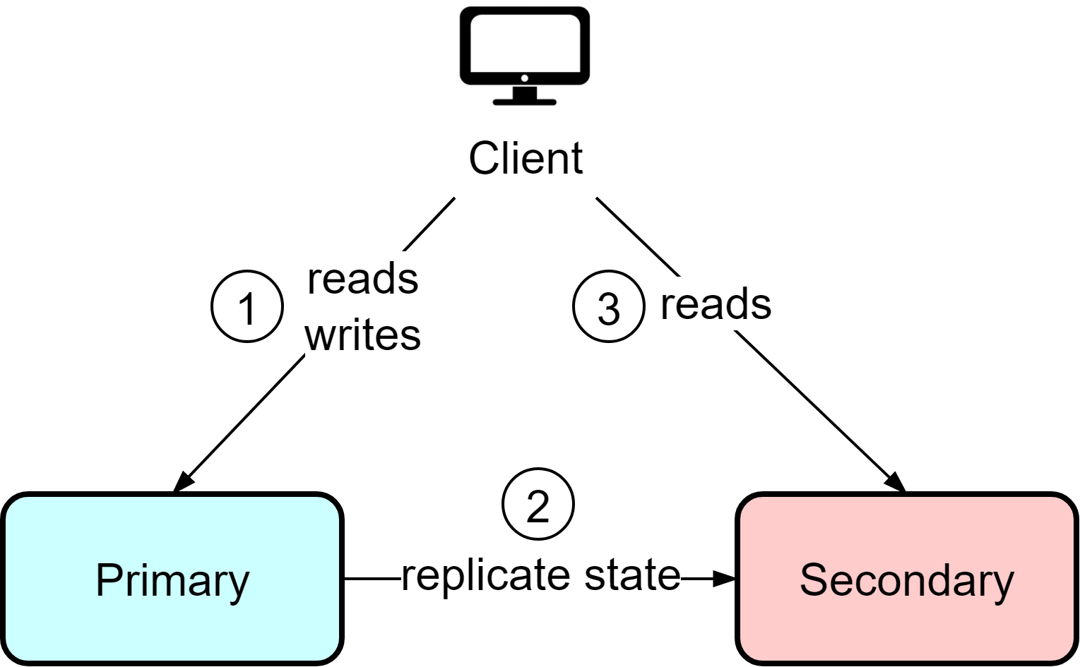
Since reads are allowed from the secondary, data consistency between the primary and secondary becomes crucial. Even if the primary instance is functioning normally, stale data could be returned from reads since requests go to both instances.
Compared with hot-cold, the hot-warm architecture is more suitable for read-heavy workloads like news sites and blogs. The tradeoff is potential stale reads even during normal operation in order to utilize resources more efficiently.
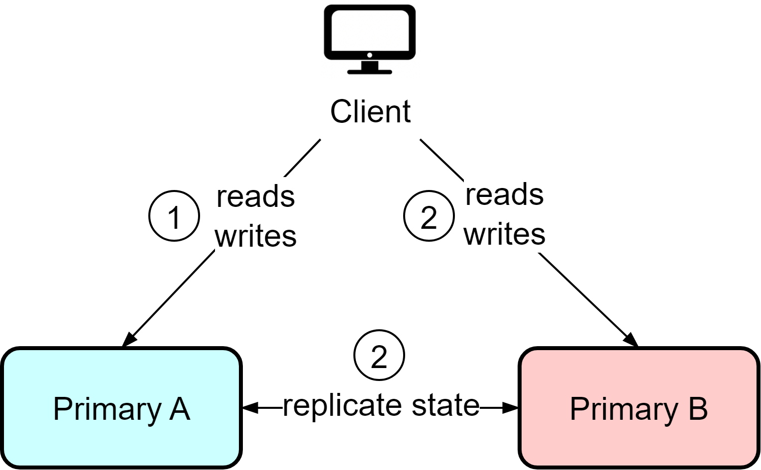
In the hot-hot architecture, both instances act as primaries and can handle reads and writes. This provides flexibility, but it also means writes can occur to both instances, requiring bidirectional state replication. This can lead to data conflicts if certain data needs sequential ordering.
For example, if user IDs are assigned from a sequence, user Bob may end up with ID 10 on instance A while user Alice gets assigned the same ID from instance B. The hot-hot architecture works best when replication needs are minimal, usually involving temporary data like user sessions and activities. Use caution with data requiring strong consistency guarantees.
In modern systems dealing with large amounts of data, two instances are often insufficient. A common scaling approach is:
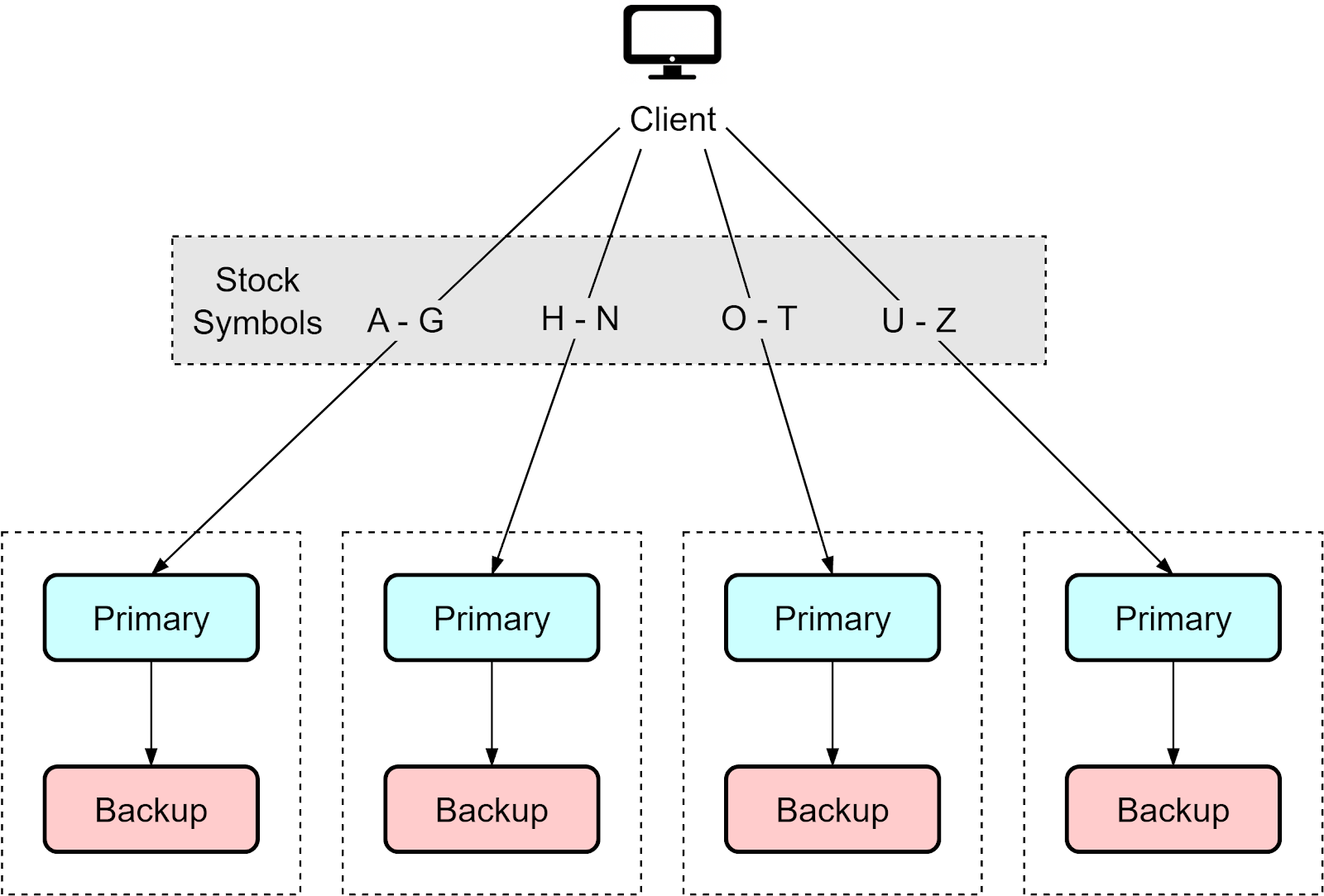
Each hot-cold pair handles one portion of the data. If the hot instance fails, its requests fail over to the cold backup containing the same subset of data. This partitioned approach simplifies the data distribution - each pair manages and backs up a segment of the overall data.
Next, let’s look at different data replication strategies. They are widely adopted in many modern storage systems.
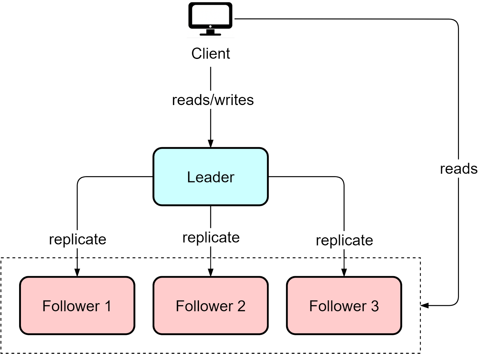
In a single leader architecture, a cluster contains multiple nodes, with one designated leader node handling all writes from clients. Replica nodes maintain copies of the leader’s data to handle reads (with a small lag). Databases like MySQL and PostgreSQL use leader-based clustering.
This redundancy helps in two ways:
Easier scalability. If we need more capacity for read queries, we can quickly provision a replica node and synchronize data from the leader instance.
Geographic caching. When supporting a global user base, we can place replicas closer to them for lower latency.
However, adding copies introduces complexity around consensus:
1. How does the leader propagate changes?
The leader focuses on processing writes. Instead of having it push changes, databases like MySQL record updated in a binlog. New replicas request this log to catch up on changes.
Replication can be asynchronous for performance or synchronous (with tunable durability guarantees) for consistency. Kafka offers both modes - we can configure the “acks” setting to be 1 or all, meaning Kafka commits the message when one replica acknowledges the replication or all replicas acknowledge.
2. What happens when the leader fails?
We need to handle three things:
a) Failure detection - A common approach is to use heartbeats every 30 seconds. If no response, the node is considered "dead".
b) Leader election - The new leader could be the node with the most up-to-date data, manually chosen by an admin, or elected via a consensus algorithm like Raft or Paxos to get an agreement.
c) Request rerouting - Once a new leader is determined, client requests need to be pointed to it. An automated service discovery layer between the clients and cluster can handle this redirection.
3. How do we handle replication lag?
There is always some lag between the leader and replicas during propagation. This can cause stale reads if not handled properly.
For example, say we update our user profile and then want to immediately check the change. The update may not have replicated yet, so reading from a repliculd give stale, inconsistent data.
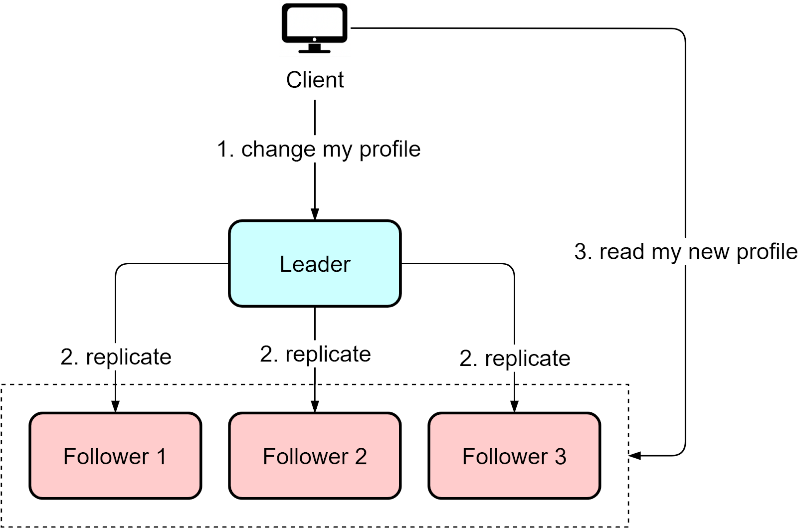
The solution is "read-after-write" consistency, where reads immediately after writes are directed to the leader. This ensures clients see the latest data.
App logic needs to account for this lag possibility to prevent anomalies. The replication delay means the data on the replicas are eventually consistent, and anomalies can occur during the propagation window.
The single-leader approach focuses on horizontally scaling reads across replicas. However, having only one node accept writes is a potential bottleneck. Some systems require higher write availability and durability across multiple nodes. Multi-leader architectures can provide increased write availability, but introduce complexity around distributed conflict resolution between the leaders, as we will see next.
The book Designing Data-Intensive Applications provides a useful example of a multi-leader architecture, where there is a leader database server in each data center that can accept write requests. WRites to one leader are replicated to follower servers in the same data center, as well as to the other leader server in the second data center. This provides high availability - if one data center goes down, the other leader can still accept writes.
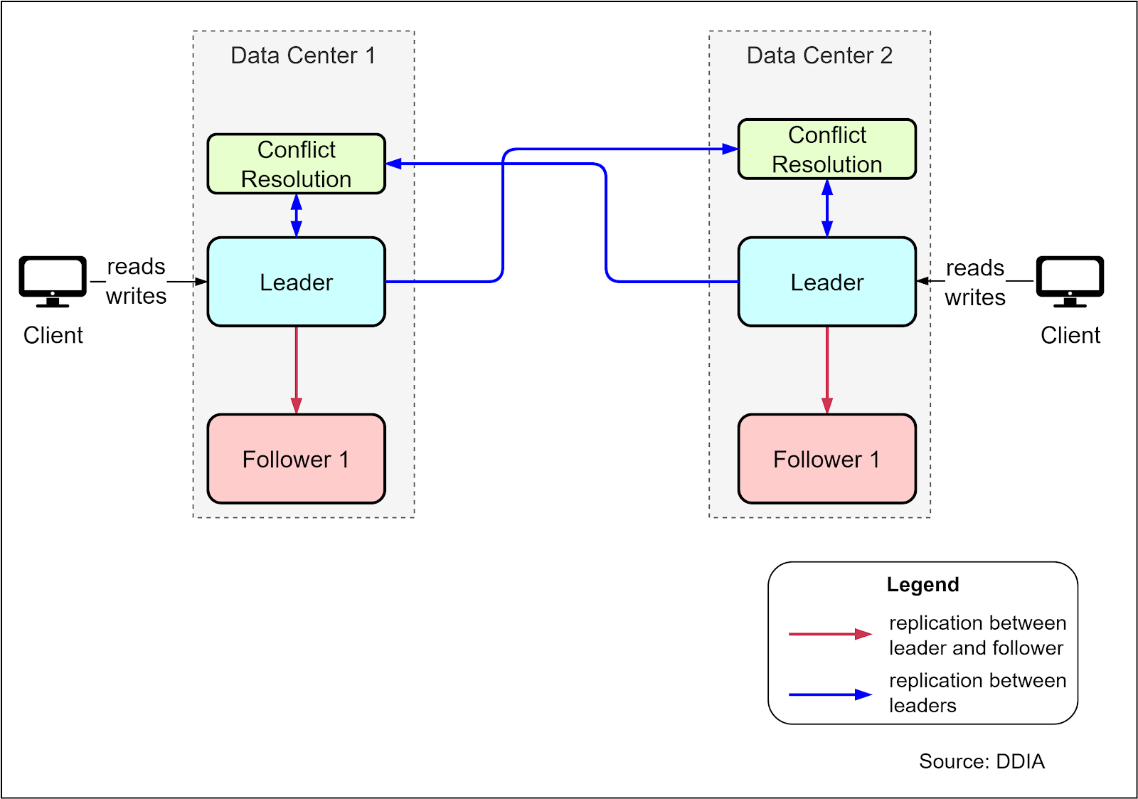
However, there needs to be an additional conflict resolution component to reconcile conflicting writes that might occur between the two leaders. This adds development effort and operational risk. The complexity of conflict resolution is a downside to weigh against the high availability benefit. Multi-leader architectures should only be considered when the high availability requirement justifies the extra complexity.
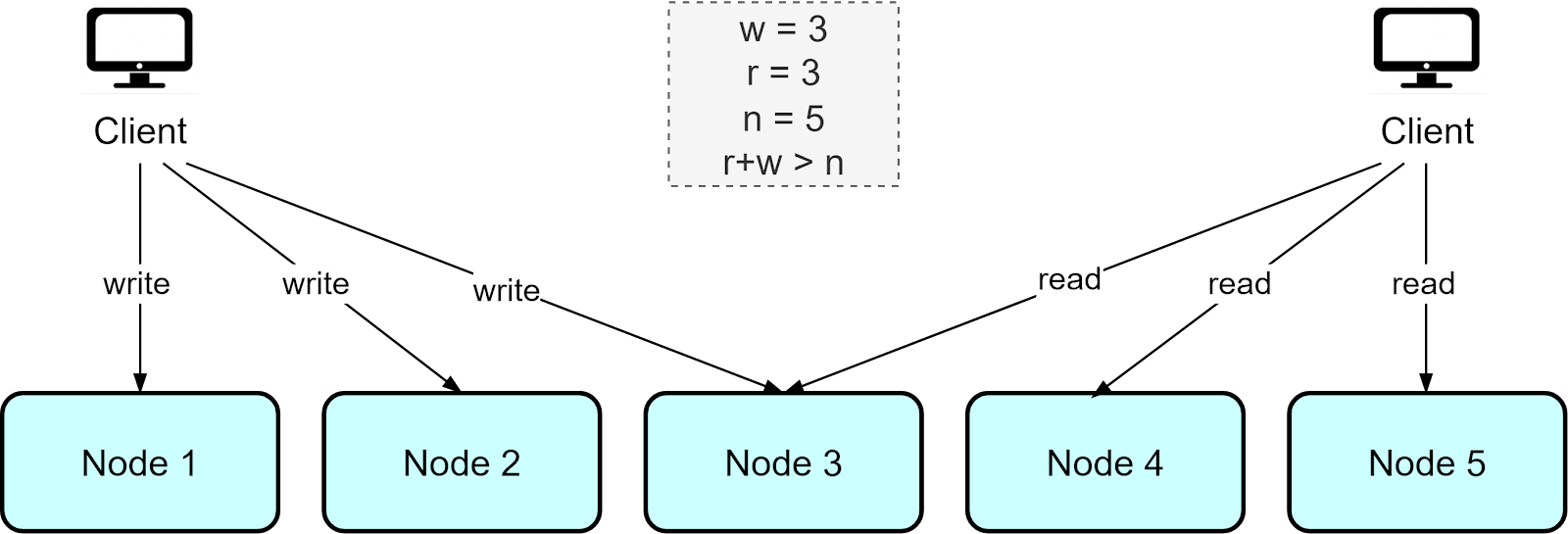
The Amazon Dynamo database uses a leaderless architecture where write requests are sent to multiple nodes (w) and read requests are also fanned out to multiple nodes (r). As long as the number of nodes written to and read from exceeds the total number of nodes, that is, r + w > n, this ensures the most up-to-date data can be read. This approach, based on quorums for reading and writing, allows maximum availability since there is no leader node
However, giving up consistent leadership introduces other complexities:
If reading from several nodes returns different versions of data, the client uses the latest version and repairs the other nodes. This “read repair” reconciles inconsistencies.
With loose consistency requirements, many data differences can accumulate between nodes. A background “anti-entropy” process continually looks for and fixes these differences.
Leaderless designs allow high availability and concurrent writes. But this comes at the cost of added complexity to detect and resolve update conflicts. There is a tradeoff between consistency guarantees and high availability.
As microservices and serverless architectures become more popular, the service layer often does not store data but serves for computation.
A “hot-hot” configuration with redundant compute nodes can provide high availability of processing capacity. If one side goes down, you simply lose half your capacity temporarily.
For large-scale computations like risk modeling, a coordinator assigns tasks to nodes in a cluster. If a node fails, the coordinator is aware and can reassign its tasks to other nodes.
By decoupling stateless application logic from stateful storage, the computation layer can scale and failover independently from the data storage, enabling flexible high availability configurations.
Adding redundancy in a system can improve reliability when dealing with failures. However, there are other mechanisms to restrict incoming load so the system is protected from traffic spikes, reducing the chance of failures.
There are four common approaches:
Rate limiting
Service degradation
Queuing
Circuit breaking
We call these tradeoffs because they sacrifice something, such as latency or services, to maintain availability.
We often restrict the number of requests to protect against sudden spikes or denial of service attacks. This is calculated based on capacity measured during performance testing. For example, during flash sales, we may only allow 100,000 concurrent users, rejecting others. We sacrifice service availability for some users to guarantee quality for the 100,000.
When under high load, we can provide only core services, removing non-essential ones. For example, a stock trading application experiencing heavy load may allow trading but not checking statements.
Unlike rate limiting, queuing allows requests to into the system, but makes them wait until previous ones finish. This sacrifices latency but increases service availability.
A circuit breaker prevents cascading failures in distributed systems. For example, if a payment service doesn’t respond within a set amount of time, the upstream order service can stop connecting to it, asking users to pay later. We sacrifice some functions in the pipeline for responsiveness and stability upstream.
In this article, we discussed the importance of designing highly available systems and typical architectures that facilitate high availability. There are three main approaches:
Add redundancies to prepare for failures.
Make tradeoffs to reduce the chance of failures.
Optimize operations and maintenance to reduce failures.
We discussed different configurations for replicating data and four common tradeoffs.
High availability is key for areas like data centers, cloud services, telecommunications, healthcare, and any field where downtime has major negative consequences. We hope this article helps you desgin more reliable systems in interviews and daily work.